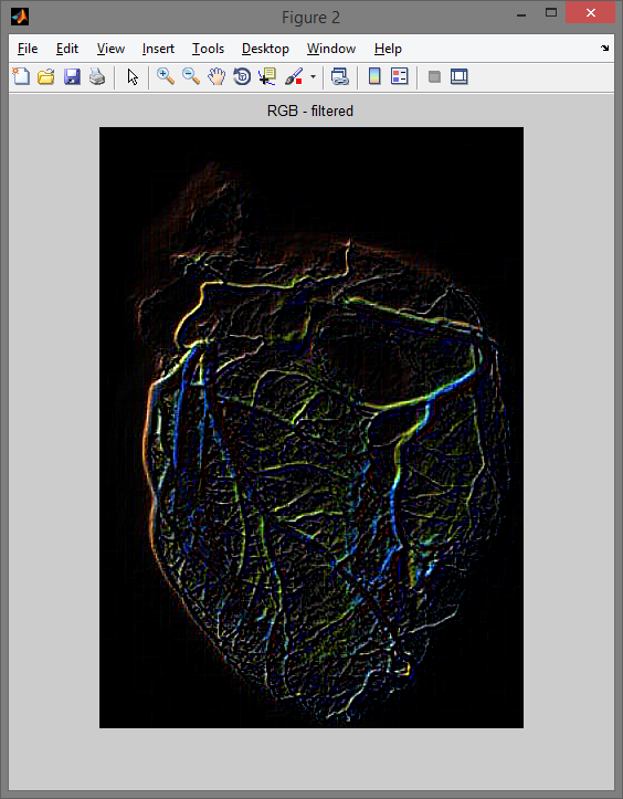
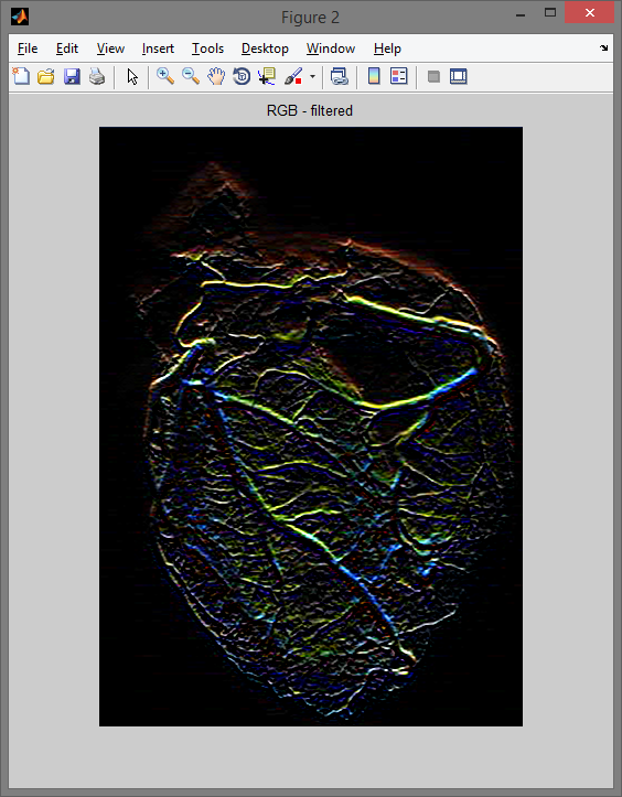
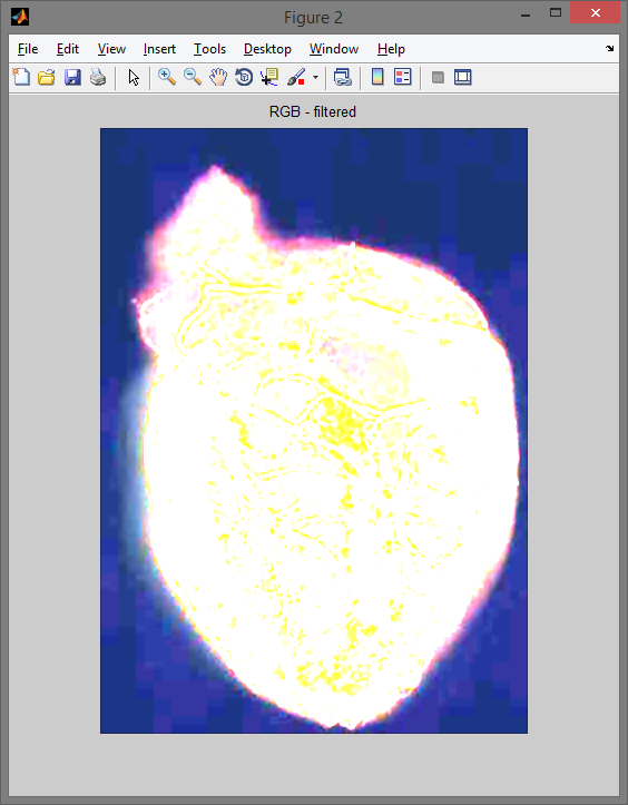
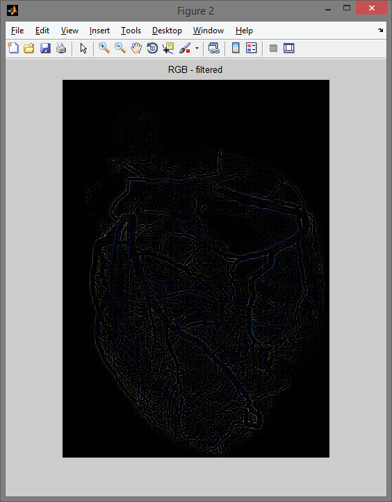
Filtry

clear all
clc
close all 

x = imread('heart_angiography','jpg');

red = x(:,:,1);
green = x(:,:,2);
blue = x(:,:,3);
a = zeros(size(x, 1), size(x, 2));
red_c = cat(3, red, a, a);
green_c = cat(3, a, green, a);
blue_c = cat(3, a, a, blue);

%% filtry uśredniające - dolnoprzepustowe
% h=[1 1 1; 1 1 1; 1 1 1];
% h=[1 1 1; 1 2 1; 1 1 1];
% h=[1 2 1; 2 4 2; 1 2 1];
% h=[1 1 1; 1 0 1; 1 1 1];

%% filtry wykrywające krawędzie
% h=[-1 -1 -1; 0 0 0; 1 1 1]; % Prewitt
% h=[-1 -2 -1; 0 0 0; 1 2 1]; % Sobel
% h=[0 0 0; -1 0 0; 0 1 0]; % Roberts

%% filtry wykrywające narożniki
% h=[-1 -1 1; -1 -2 1; 1 1 1]; 
% h=[-1 -1 -1; 1 -2 1; 1 1 1];
% h=[1 1 -1; 1 -2 1; 1 1 -1]; 
% h=[1 1 1; 1 -2 1; -1 -1 -1]; 

%% filtry specjalizowane
%h=fspecial('gaussian');
%h=fspecial('disk');
%h=fspecial('laplacian');
%h=fspecial('prewitt');

%h=zeros(size(x));
y = zeros(size(red));
y = uint8(filter2(h,red));

y1 = zeros(size(green));
y1 = uint8(filter2(h,green));

y2 = zeros(size(blue));
y2 = uint8(filter2(h,blue));

red_filtred = y(:,:,1);
green_filtred = y1(:,:,1);
blue_filtred = y2(:,:,1);
rgb_filtred = cat(3, red_filtred, green_filtred, blue_filtred);

subplot(221);imshow(x); title('RGB');
subplot(222);imshow(red_c); title('R');
subplot(223);imshow(green_c); title('G');
subplot(224);imshow(blue_c); title('B');
figure,imshow(rgb_filtred); title('RGB - filtered');

subplot(131); imshow(x); title('Obraz wejsciowy');
subplot(132); imshow(h); title('Obraz Filtr');
subplot(133); imshow(y); title('Obraz po filtracji');